I’m a geophysical fluid dynamicist. I want to understand how the ocean’s small scales (eddies, waves, and turbulence) shape its large-scale circulation and, through that, the climate. I combine theory, idealised models of increasing complexity, and realistic simulations. A big part of my effort goes into building new open-source, GPU-native ocean and climate models. With these, the gap between theory and simulation in climate science gets narrower, because the simulations we can run get closer to the questions we want to ask.

Southern Ocean and the Antarctic margin

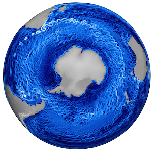
Credit: NASA/JPL

The Antarctic Circumpolar Current (ACC) is the largest current in the ocean. It connects all ocean basins and plays a central role in the climate by setting up the meridional overturning circulation and controlling how heat and carbon move around the ocean. The westerly winds that drive the ACC have strengthened and shifted polewards in recent decades.

How does the ACC respond to stronger winds? Observations and eddy-resolving models suggest that its transport is remarkably insensitive to wind changes, a phenomenon known as eddy saturation. Using conceptual models of increasing complexity, from quasi-geostrophic turbulence on a beta plane above topography to a primitive-equation channel model, I’ve worked to delineate the roles of barotropic and baroclinic processes, and of bathymetry, in the ACC’s response to changing winds. The Southern Ocean’s eddy field is also strongly chaotic, and its intrinsic variability differs markedly around the continent.

Closer to Antarctica, the Antarctic Slope Current acts as a barrier between the warm Circumpolar Deep Water offshore and the floating ice shelves. We showed that warm water can cross this barrier through submarine canyons in intrinsically episodic intrusions, even under steady forcing. We also showed that meltwater from Antarctica can transiently weaken the Slope Current, which may open the door for more warm water to reach the ice (read more in The Conversation).

These processes span scales from the circumpolar current down to bottom mixing and surface waves. We review how they connect in Closing the loops on Southern Ocean dynamics (read more in The Conversation).

Parametrisations: physics-informed and data-driven

Credit: GFDL

Climate projections require simulations hundreds of years long, so climate models cannot afford to resolve every scale of oceanic motion. Instead, they rely on parametrisations: models for the collective effect of unresolved motions on the scales the model does resolve. Better parametrisations come from understanding the underlying dynamics, and increasingly from learning from high-resolution data.

With the ocean team of the Climate Modeling Alliance (CliMA), we developed CATKE, a one-equation parametrisation for vertical mixing in the ocean’s surface boundary layer. Its free parameters are calibrated automatically against large-eddy simulations using Ensemble Kalman Inversion, with tools like ParameterEstimocean.jl. This approach, physics-based closures whose parameters are learned from data, is how I think parametrisations should be built: interpretable, but systematically constrained by high-fidelity simulations.

Supported by a Discovery Early Career Research Award from the Australian Research Council (awarded in 2021), I’ve also been developing data-driven, physics-informed parametrisations for the ocean’s mesoscale eddy fluxes, using output from eddy-resolving models together with machine-learning methods. Beyond eddies and boundary layers, we have also evaluated and improved parametrisations of wave and non-wave stresses that arise when oceanic flows interact with rough bathymetry.

Read more about how machine learning can enhance the accuracy of climate and ocean models in The Conversation.

Climate variability

Not all ocean variability is forced by the atmosphere. A significant part is intrinsic: it emerges from the ocean’s own nonlinear, eddying dynamics. We showed that this intrinsic ocean variability contributes substantially to decadal variations in upper-ocean heat content, and can then feed back onto the atmosphere through air–sea interactions. This is something coupled climate models that do not resolve mesoscale eddies cannot capture.

Trends in surface eddy kinetic energy, 1993–2020.
Credit: Martínez-Moreno et al. (2021)

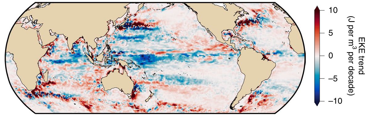
The ocean’s mesoscale is also changing. Using a framework for estimating the kinetic energy of eddy-like features from satellite altimetry, we found global changes in oceanic mesoscale currents over the satellite altimetry record: eddy kinetic energy has increased in many energetic regions of the ocean over the past few decades (read more in The Conversation).

At the scale of ocean basins, I’m interested in how modes of climate variability shape the climate far from where they originate. For example, we have been characterising the diversity of La Niña events and their impacts on Pacific teleconnections.

Next-generation ocean and climate models

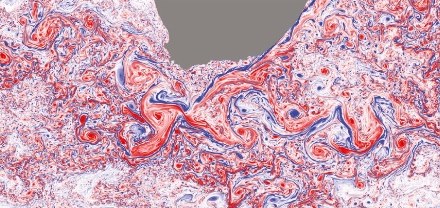
Surface vorticity in the Agulhas region from a 1/48° near-global Oceananigans simulation.
Credit: Silvestri et al. (2025)

How well we understand the climate is limited by the simulations we can afford to run. Over the past few years, a large part of my work has been building a new generation of open-source ocean and climate model components in Julia. These components are designed from scratch to run on GPUs and to be easy to use, extend, and couple to data-driven tools.

I’m one of the core developers of Oceananigans, a library for ocean simulations at all scales, from large-eddy simulations of boundary-layer turbulence to global ocean models. Oceananigans’ GPU-based hydrostatic dynamical core makes mesoscale-resolving global ocean simulations routine rather than heroic. Getting there also needed new numerics, such as a WENO-based momentum advection scheme tailored to mesoscale turbulence and a low-storage Runge–Kutta framework for nonlinear free-surface ocean models. I’ve also contributed to OceanBioME, for coupled ocean biogeochemistry and physics.

NumericalEarth: a framework for Earth system modelling

Models that simulate different aspects of the Earth system become far more powerful when they are coupled together. I’m a co-owner of NumericalEarth, where we are building NumericalEarth.jl, a new framework for Earth system modelling at all scales. NumericalEarth.jl couples ocean, sea ice, atmosphere, and land components, each of which can be either prognostic or prescribed from observations and reanalyses, and computes the fluxes between them. Oceananigans provides the ocean. The atmosphere can be the general circulation model SpeedyWeather.jl, to which I’ve also contributed, or Breeze.jl, a GPU-native atmosphere model built on Oceananigans that spans large-eddy simulations up to the mesoscale. For the land, we are developing Terrarium.jl, a framework for differentiable, GPU-accelerated land and ecosystem models. Because every component is written in Julia and designed for GPUs from the start, the coupled model is meant to be as easy to set up and extend as any of its components on its own.

Air–sea interactions and coupled modelling

The ocean and atmosphere constantly exchange momentum, heat, and freshwater, and many of the questions above, from intrinsic variability to the response of the Southern Ocean to changing winds, are fundamentally coupled problems. Coupling Oceananigans and Breeze lets us run atmosphere–ocean large-eddy simulations in which the turbulent boundary layers on both sides of the air–sea interface are resolved explicitly. We use these simulations to understand how the atmospheric and oceanic boundary layers evolve together, and how momentum, heat, and freshwater are exchanged between them. Climate models have to parametrise these exchanges, and NumericalEarth.jl doubles as a sandbox for developing and testing the air–sea flux parametrisations they rely on.

See the software page for more.

Earlier work: turbulence and coherent structures

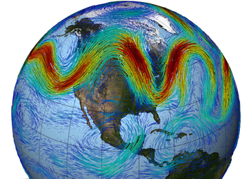
Credit: NASA GSFC

Statistical state dynamics of jets. Planetary atmospheres self-organise into large-scale coherent structures, such as Earth’s jet streams, that are maintained by the turbulence they coexist with. Classical stability analysis assumes that a mean state exists without the fluctuations, so it can’t describe these structures. In my doctoral thesis and afterwards, I used Statistical State Dynamics (SSD), the dynamics of the flow statistics themselves, to predict how homogeneous turbulence self-organises into jets, the mechanism behind this self-organisation, how jets equilibrate at finite amplitude, and how jets, large-scale waves, and turbulence coexist.

Gas giants. With Jeffrey Parker, we showed that magnetic fields in the interior of gas giants can suppress the formation of zonal jets, and that turbulent magnetic fluctuations act on the mean flow as an effective “magnetic viscosity”. This mechanism offers a plausible explanation for the depth of the jets on Jupiter and Saturn revealed by Juno and Cassini.

Wall-bounded turbulence. With Adrián Lozano-Durán and others, we studied very-large-scale roll–streak motions in channel flows. We also showed that the modal instabilities of streaks are not the main route by which energy is transferred to turbulent fluctuations, and probed the cause and effect of the linear mechanisms sustaining wall turbulence.